As a psychologist with a background in the natural sciences, I have always preferred accounts (“models”) of psychological phenomena which draw upon a mathematical or computational framework. There was a nice example of this approach to psychological model building in an earlier entry in the departmental blog by Caspar Addyman. (1). When so much psychological theorising is expressed using simple (and often ambiguous) qualitative verbal arguments, those who turn to mathematical psychology have sometimes been accused of “physics envy”, I would rather think of it as a preference for trying to understand things using “the language that nature speaks in”, as the Nobel Prize winning physicist, Richard Feynman, once said.

The Drift-Diffusion Model

A recent article by Ratcliff et al (2016) provides some interesting insights into how mathematical models, drawn from physics, may contribute to understanding psychological processes. This article reviewed the vast array of evidence that has accrued, over four decades, to support the so-called “drift-diffusion” model (DDM) of speeded choice. The DDM is used to account for the speed and accuracy of responses made to stimuli. It is directly derived from the physics that describes the partly random diffusion of small particles in a fluid (so-called “Brownian motion”; you might remember learning about this in high school science classes).

The DDM is based on relatively simple mathematics. The model equations track the position of a “particle” as a function of continuous time. The simplest case is to consider a particle which can move along a line, for example by moving up or down. The particle is influenced by two processes which affect the way it moves. First, it is continuously buffeted by random diffusion movements which move it upwards one moment and then downwards the next. As this process is random it does not move the particle in any particular direction: the average position of the particle just stays put, where it started. In addition, the particle has a characteristic rate of drift which is a steady movement, either up or down.

Psychologists have used the DDM model to study choice reaction times (RTs) by considering how long it might take the particle to collide with one of two barriers (or decision boundaries). The barriers are equidistant from the particle’s staring position: in our example one barrier is a fixed distance above the particle, the other the same distance below. Each barrier represents a decision point corresponding to one of the choices in a two-choice task. The “times to collision” of the particle, with these barriers, are taken (after suitable rescaling) to be the model of the RTs. More precisely, the collision times reflect the decision, or choice, part of these RTs. The time taken to encode stimuli and the time for executing the response after deciding which response to make are captured as a simple random variable and added to the choice component captured by the diffusion equations.

Drift-Diffusion and Reaction Time Studies

We will consider some basic questions about this popular and influential model: what features of choice RT data is it able to model, which model features (assumptions) are critical to the model’s ability to capture aspects of the data, and is the use of this particular physical model necessary, sensible and appropriate for capturing patterns in RT data?

It is easier to imagine this model with time divided into discrete timesteps, in which case it is strictly called a random walk model. Here I will describe a simple version in which the particle moves up or down the rungs of a ladder (see Figure 1). Imagine the ladder has 501 rungs and, on each trial of the psychological task being modelled, let us assume that the particle starts midway up the ladder at rung 251. Imagine also that each trial of the task being modelled involves seeing a picture of a face posing either a happy or fearful expression, and the participant has to identify the emotional expression on each face quickly and accurately using button-press responses. The model allows one to track the movement of the particle over timesteps on each trial. We can decide (arbitrarily) that a response of “happy” will be given whenever the particle reaches the top rung of the ladder, and “fearful” whenever it reaches the bottom. Note that the number of timesteps taken to reach one or other of these response thresholds will be used to capture the decision time on that particular trial.

The movement of the particle up and down the rungs is essentially a means for expressing the rate of information gathering in the direction of each response (upwards=happy; downwards=fearful). Imagine on each discrete step of time the particle moves either 10 rungs up the ladder or 10 rungs down, determined at random with a 50:50 chance of moving in either direction. Clearly, this just adds noise and variability to the timing of the movements, and thus to the response decisions. This random diffusion process will, on average, move the particle neither up nor down. Participants generally respond correctly and so the model needs a means for ensuring that, on happy face trials, the particle generally moves in an upward direction (and downward on fear face trials).  To do this, the model uses the drift rate. One can set the drift rate by saying, for example, that the particle will move 1 rung of the ladder on each timestep in a constant direction. A faster drift rate (in rungs moved per timestep) will give faster response times. The drift direction will be in the correct direction (on correct response trials) and in the wrong direction (on error trials).

In a task where a participant makes 95% correct responses, one can determine the drift rate, on a particular trial, by using a biassed coin with a 95% chance of landing heads. On happy face trials, when the coin comes up heads, the particle moves one rung up the ladder on every timestep. On fear face trials, a heads outcome moves the particle one rung down the ladder on every timestep. As a result the particle will gradually, yet noisily, move in the correct direction on 95% of the trials and in the wrong direction on 5% of the trials. Once can change the bias of the coin used to capture the different levels of error made in different tasks and/or by different participants. Figure 1 shows an example of two trials with correct responses.

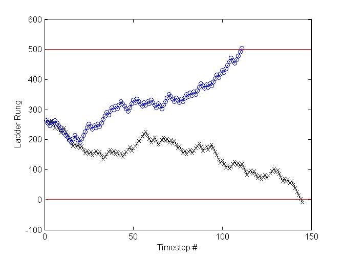
Figure 1: The random walk of the particle on a simulated happy face trial (blue circles) and a fear face trial (black crosses). Note the decision component of the RT is modelled by the number of timesteps to reach the top or bottom of the ladder (red lines). The trial decisions completed in 111 (happy) and 145 (fear) timesteps respectively.

 

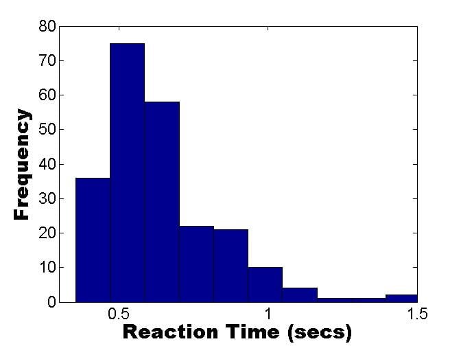
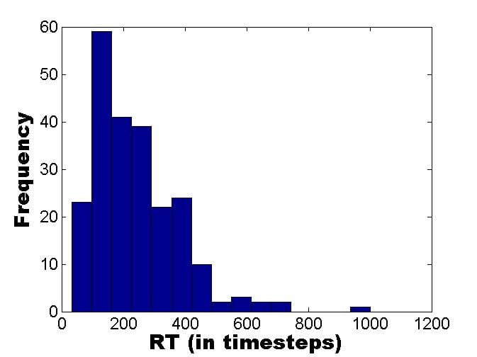
What can one simulate with this model? Let us start with the RT distribution for a single participant’s correct responses. The characteristic RT distribution for a single participant, on a wide range of 2-choice tasks, typically looks something like that shown in Figure 2A (i.e. the distribution is positively skewed). These real data were taken from a subject discriminating happy from fearful facial expressions (total trials=240). A simulation of 240 trials was run with a 5% error rate. For the correct responses (95% of trials), the simulated RT distribution for a single participant, was as depicted in Figure 2B. We can see from the Figure that the model does a pretty good in simulating the shape of the RT distribution for correct responses. Recall that we have to scale the decision timesteps into milliseconds and then add a time for the combined duration of stimulus encoding and response execution, in order to complete the modelling.

A

B

 

Figure 2. A: Real RT data (correct responses only) from a participant discriminating happy vs. fearful facial expressions. B: Simulated decision times using the ladder rung random walk version of the DDM, described above (drift rate simulated using a biased coin toss, with probability of heads=0.95).

However, the above model predicts the same RT distribution for correct and error responses. This is because the drift rate is the same (1 ladder rung per timestep) for both correct and incorrect responses; it is just the direction of the drift that changes. The typical picture in choice RT tasks is that error responses have a slower mean response that correct responses, so the assumptions of the above model must be changed in order to capture this observation. The usual way this has been done has been to allow the drift rate to vary from trial to trial. In the current ladder model this could be done by using a normal distribution to randomly determine the size of the drift on each trial. The mean of this distribution would be in the correct direction (on each timestep moving on average, say, 2 steps up for happy face trials and 2 rungs down for fear face trials). However, there would be variability across trials (e.g., a standard deviation of 1.1 rungs across trials). The value for a particular trial would be rounded to the nearest whole number of rungs. Figure 3 shows what such a distribution of drift rates would look like.

To understand why this model feature gives slow errors one should note that the (blue) happy face trials with negative drift rates in Figure 3 will lead to errors. By contrast, the majority of the happy face trials have positive drift rates and will lead to correct responses. The mean drift rate on the correct trials (with positive drift rates) is 2.26 rungs per timestep for the blue distribution shown in Figure 3, and the mean of the negative drift rates (error trials) is -0.29. Thus, the correct trials drift faster than the error trials and so the time for the correct trials to reach the top rung of the ladder (the decision criterion) is quicker than that for the incorrect trials to reach the bottom rung of the ladder. The same arguments apply equally to the (red) fear face trials in Figure 3.

 

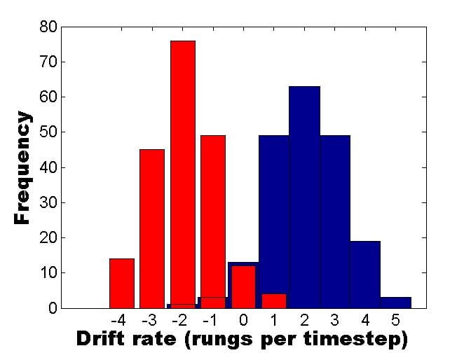
Figure 3. Variability in drift rate over trials. There are 200 happy face trials (blue) and 200 fear face trials (red). Positive drift rates indicate rungs moved up the ladder on each timestep, negative drift rates indicate rungs moved down.

However, on some tasks (such as the face emotion recognition task in my lab, the errors are consistently faster than the correct responses. This tends to happen when tasks are easy and participants are encouraged to respond rapidly. If one were to try to model this using the model we have developed so far, then one would need a bimodal distribution of drift rates for each type of stimulus. For happy face trials there would need to be a mode with positive drift rates and a mode with negative drift rates. The drift rates values in the positive mode, on average, would need to have smaller absolute values than the values in the negative mode. In this way the error trials would drift to their decision criterion (the bottom rung, for happy faces) faster than the correct trials drift towards the top rung of the ladder. This type of assumption in the model doesn’t seem very appealing to me, as it merely captures the effect without offering any explanation for what is different between a task with slow errors and the rarer task with fast errors. Why should the drift rate distributions differ?

DDM modellers capture slow errors by changing another modelling assumption. Note that so far, the ladder model has the particle always starting midway between the top and bottom rungs. In the full DDM the start position is also allowed to vary between trials, and introducing this feature into the model captures slow errors. If the start point is nearer the correct decision boundary (e.g., nearer the top rung for a happy face trial) then there won’t be many errors on these trials and they will be slow as there is a long way to drift. However, if the start point is nearer to the wrong decision boundary then there will be relatively more errors arising on these trials and they will be fast as the (wrong) boundary is relatively close. With drift rates and start points varying between trials, modellers can get the model to switch between fast and slow errors simply by closing (or widening) the gap between the decision boundaries (varying the number of rungs on our ladder).

Recently, it has been argued that these across trial variability assumptions (in drift rate, and in particle starting position) used by the DDM, make it so flexible that it can accommodate almost any result, rendering it unfalsifiable (Jones et al., 2014). In the same issue of Psychological Review, you can read a defence of the falsifiability of the DDM and related models (Smith et al., 2014 and Heathcote et al., 2014), and the response to this defence. It’s an entertaining piece of intellectual ping pong!

A final observation came from a mathematician I know who studies the maths of branching processes like those underlying the DDM. She said:

“the underlying physics is completely irrelevant to the model; you just need to know the distributions of the time-to-collision with the barriers, these distributions need have nothing to do with diffusion and drift”.

We have seen above that these distributions (of drift rate, which determine the times to collision) are a key to how the model captures the data. She further argued that to be a “real model” there would need to be something in the physics of the brain mechanisms underlying the choices made which was close to real physical diffusion processes. Interestingly, recent work has tried to fill that gap by showing that neural firing rates behave in similar ways to the physics of diffusion as captured by the DDM (see Ratcliff et al.,2016, Box 3).

The (Failed) Physics of Positivity

I think the above shows that the importance of the underlying physical model for the predictions based on the DDM is (at best) arguable. From time to time, however, psychologists have clearly overstepped the mark in using physics to develop their mathematical models of behaviour. In a series of papers, culminating in a paper in the prestigious journal, American Psychologist, Fredrickson and Losada (2005) claimed to have used non-linear dynamical equations describing the physics of chaos to uncover an emotional “positivity ratio”, which they claimed had important properties for people’s wellbeing. Their positivity ratio is the number of positive emotions exhibited by a person (or couple, or group of people) divided by the number of negative emotions they exhibited. Friedrickson and Losada claimed that the mathematical model predicted that individuals “flourish” when this ratio exceeds 2.9 (but is below 11.6). The concept represented by the non-linear equations was that when the positivity ratio was below 2.9 the individual is in one state (non-flourishing; imagine this being akin to ice) and that as the positivity ratio reaches the “tipping point value” of 2.9, their full potential is suddenly released (akin to them transitioning suddenly to another state, like liquid water).

The claims in the 2005 paper, at surface value, sound important and the underlying mathematical model and equations must have appeared impressive. These factors seem likely to have been part of the reason why this paper had received 322 citations between its publication and April 2013. However, the validity of the use of this mathematical model severely troubled a part-time masters student from the University of East London, Nick Brown, who was studying the 2005 paper as part of a module on “positive psychology”. He contacted an academic called Alan Sokal whom he felt might be able to help him write a paper criticising the earlier work on the positivity ratio. They subsequently published their critique in the same journal (Brown et al., 2013). The abstract of their critique perfectly summarises both the issues with this particular piece of pseudo-science and some general guidance on the use of mathematical modelling tools in psychology:

“We examine critically the claims made by Fredrickson and Losada (2005) concerning the construct known as the “positivity ratio.” We find no theoretical or empirical justification for the use of differential equations drawn from fluid dynamics, a subfield of physics, to describe changes in human emotions over time; furthermore, we demonstrate that the purported application of these equations contains numerous fundamental conceptual and mathematical errors. The lack of relevance of these equations and their incorrect application lead us to conclude that Fredrickson and Losada’s claim to have demonstrated the existence of a critical minimum positivity ratio of 2.9013 is entirely unfounded. More generally, we urge future researchers to exercise caution in the use of advanced mathematical tools, such as nonlinear dynamics, and in particular to verify that the elementary conditions for their valid application have been met.” (Brown et al., 2013, p. 801)

A full treatment of this bizarre case is given in a 2015 lecture by Alan Sokal. His devastating critique of the published “positivity ratio” papers is an entertaining read, by turns jaw-dropping and hilarious, despite being a sad indictment of the academic peer reviewing process that allowed the 2005 paper to be published in the first place. This point was put rather punchily in slide 228 of his lecture: “How could such a loony paper have passed muster with reviewers at the most prestigious American Journal of Psychology?” How indeed!

Prof. Alan Pickering reacts to tweets according to an as yet undermined mathematical model  @ad_pickering.